How to use ANSYS on LiCO

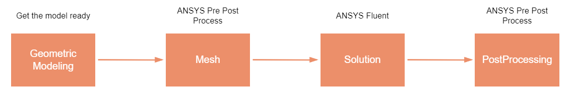
This guide will demonstrate the use of ANSYS based on LiCO

ANSYS Usage Process, Taking Fluent as an Example

Workflow

• ANSYS Fluent Preprocessing : Mainly responsible for importing modeling files, meshing the modeling, setting solution parameters for the meshed files, and saving the processed .cas files
• ANSYS Fluent Solution : Calculate and get the solved files, based on the files processed by the ANSYS Fluent Preprocessing operation
• ANSYS Fluent Postprocessing : Import the .cas file solved by the ANSYS Fluent Solution step, and perform post-processing to get the ideal renderings and parameters

ANSYS Fluent Preprocessing

1. Open and Log in LiCO, Select ANSYS Template

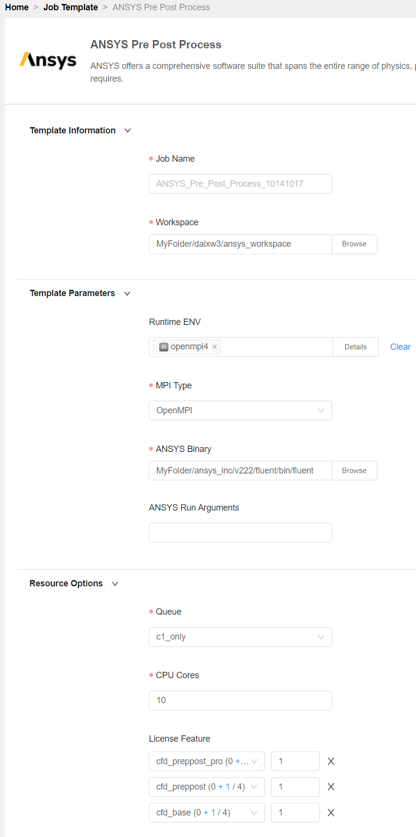
Job Template → ANSYS Pre Post Process

2. Fill in the Job Parameters

• ANSYS Binary : ANSYS startup file
• ANSYS Run Arguments ：Extra parameters at ANSYS startup

3. Start ANSYS Fluent With VNC

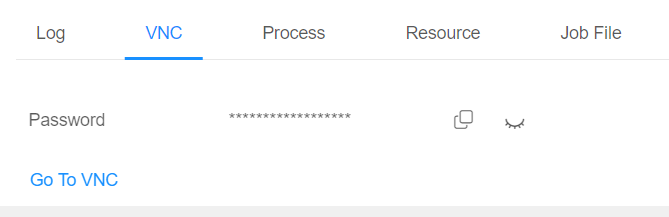
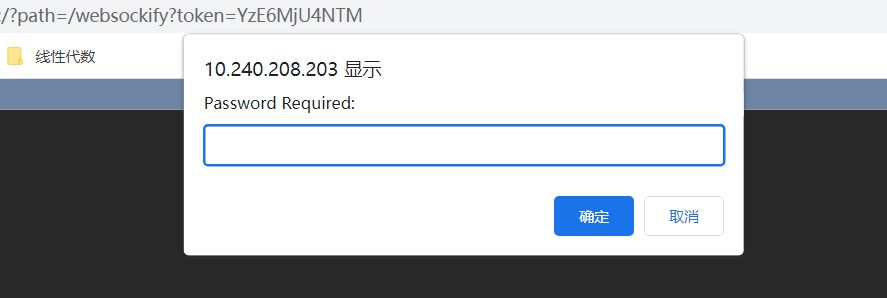
After the job runs normally, there will be a VNC option in the job details interface. After copying the password there, click Go To VNC, and enter the copied password in the newly popped up VNC window. After successfully entering the VNC interface, you can operate Fluent Launcher.

4. Set the Parameters of Fluent Launcher

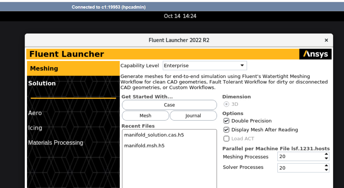
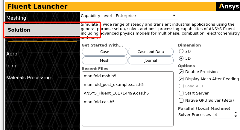
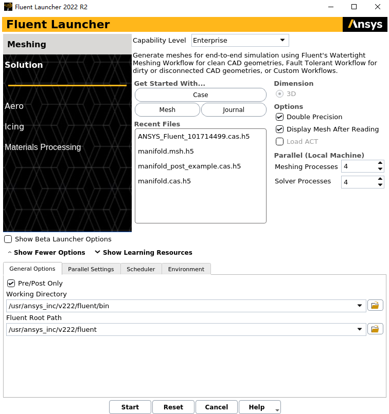
In the Fluent Launcher interface, you can choose to configure a series of parameters, including Capability Level, General Options, Parallel Setting, Scheduler, Environment, etc. After configuring the required parameters, click the Start button.

Save the .msh and .cas files after Preprocessing as the requirement files for subsequent solution and post-processing.

For detailed examples see：ANSYS Fluent Preprocessing Example

ANSYS Fluent Solution

1.Open and Log in LiCO, Select ANSYS Template

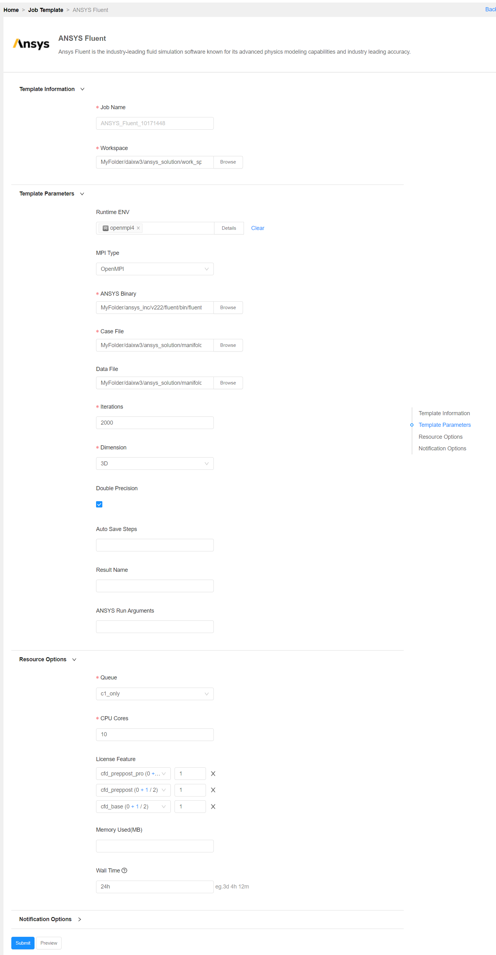
Job Template → ANSYS Fluent

2.Fill in the Job Parameters

• ANSYS Binary : ANSYS startup file
• Case File ：Solution case file (.cas.h5 file or .cas file)
• Data File ：Solution data file (.data.h5 file or .data file)
• Iterations ：The number of iteration steps required to solve
• Dimension ：Solve the dimensions of the model, 2D or 3D
• Double Precision ：Whether to enable double precision (default double precision)
• Auto Save Steps ：The step size is automatically saved, and the file will be automatically saved according to the settings during the solution process
• Result Name ：Rename the output file (defaults to Job Name as the output file name)
• ANSYS Run Arguments ：Extra parameters at ANSYS startup

3.Run the Job and Get the Solved File

If the Solution job is running properly, you can find the number of job steps on the Log page.

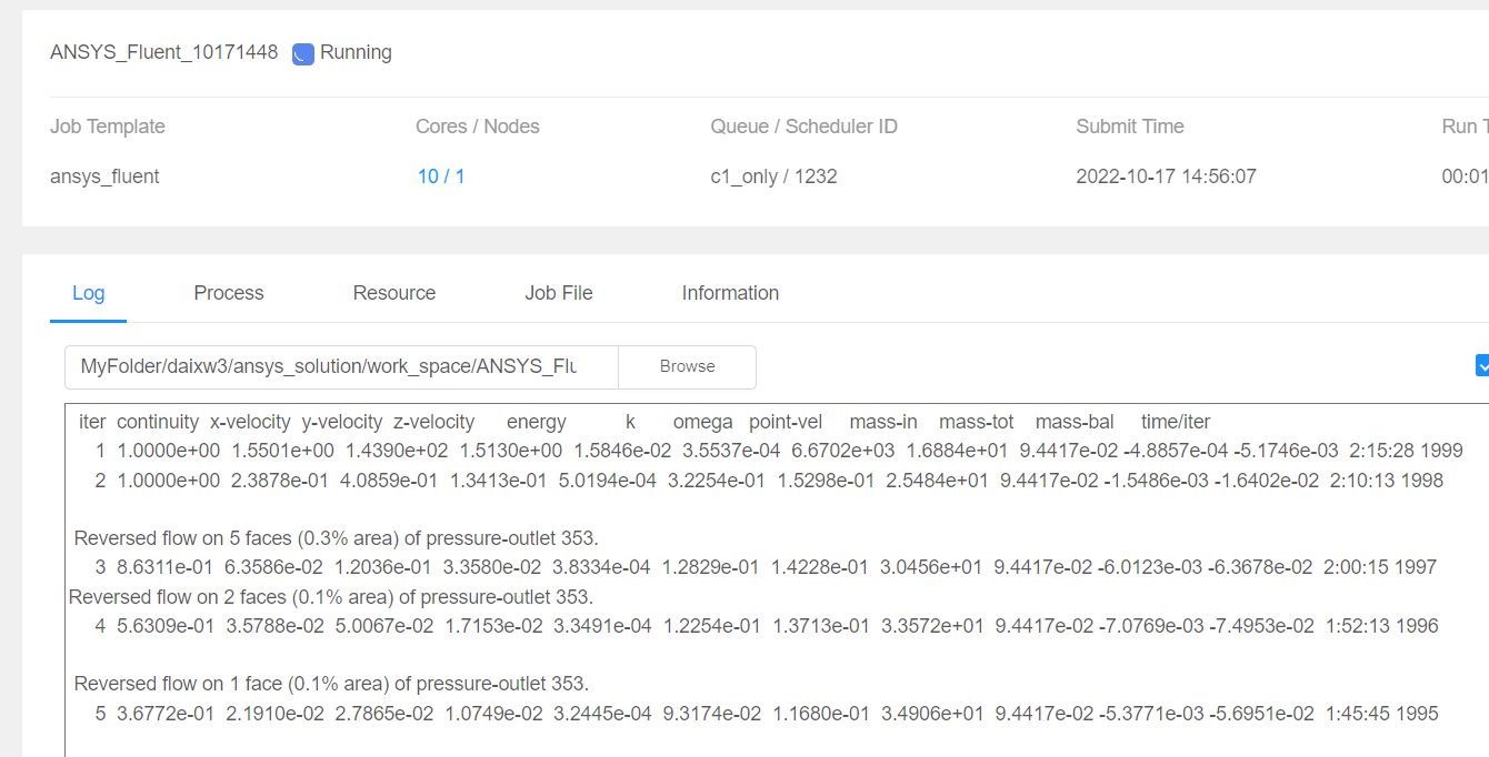
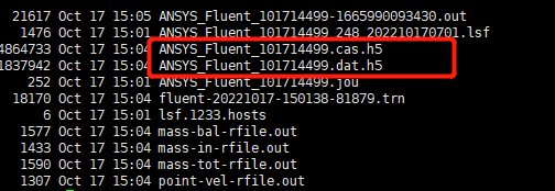
After the job runs normally, .cas.h5 and .data.h5 files will be generated in the Workspace directory. If Auto Save Steps is set, a series of result files will be generated.

ANSYS Fluent Postprocessing

Starting Fluent Launcher is the same asANSYS Fluent Preprocessing

Start in Solution Mode

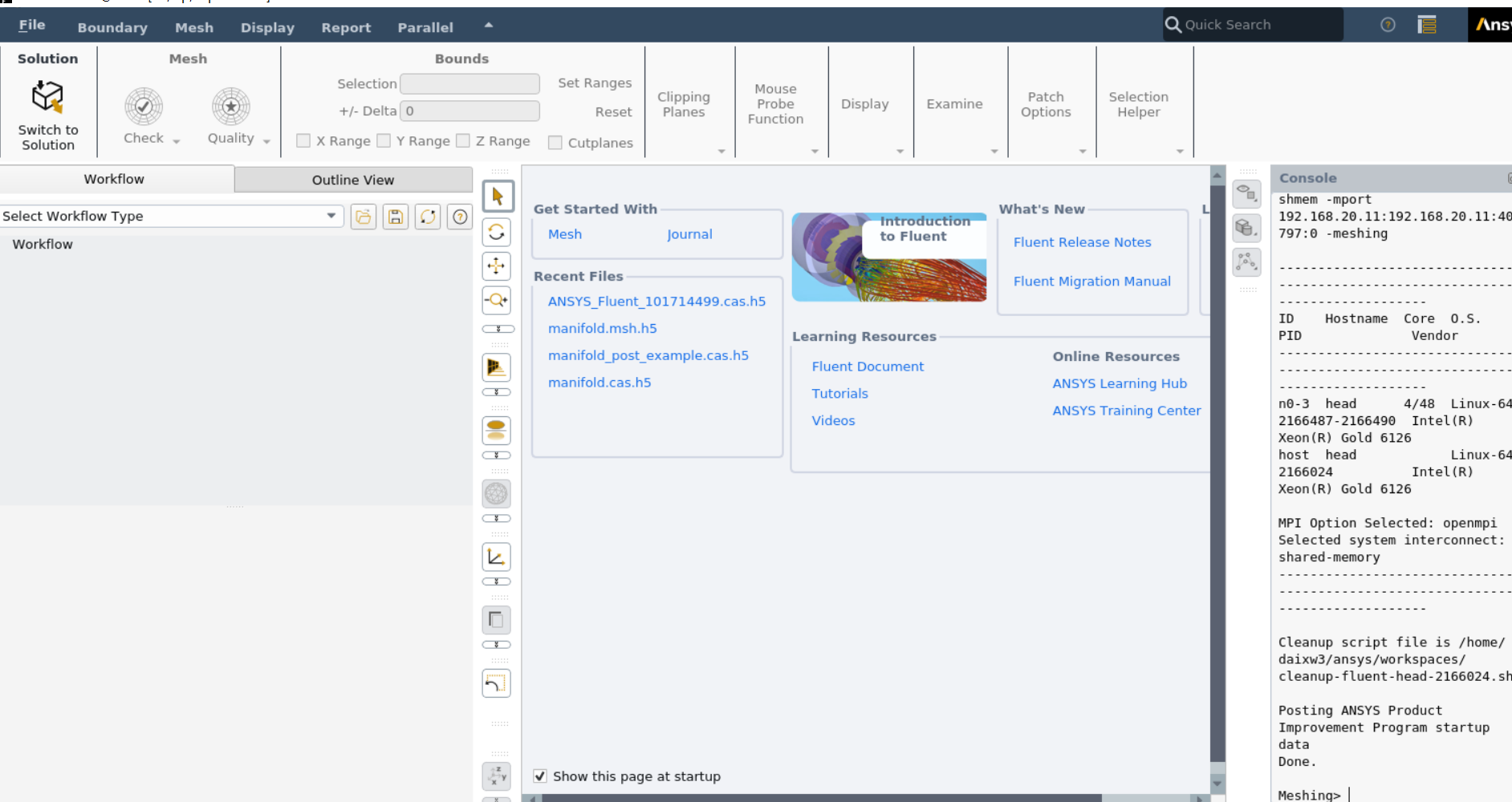
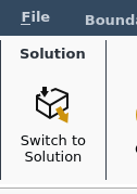
In the Fluent Launcher interface, you can select Solution to start, and directly enter the Solution mode for postprocessing. If you start in Meshing mode, you can also select Switch to Solution mode on the Fluent program page.

Import Files for Postprocessing

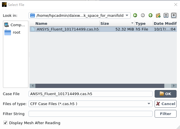
After starting the fluent program, import the .cas.h5 file generated by the Solution for some postprocessing.

File → Read → Case&Data

For detailed examples see：ANSYS Fluent Postprocessing Example

Example

ANSYS Fluent Preprocessing Example

Start Fluent Launcher

1. Ensure that the proper options are enabled

a. Ensure that the Double Precision option is selected.

b. Ensure that the Display Mesh After Reading option is enabled.

c. Set Processes to 4 under the Parallel (local Machine).

Note:

Fluent will retain your preferences for future sessions.

2. Set up your own working directory

a. Click the Show More Options button to reveal additional options.

b. Enter the path to your working folder for Working Directory by double-clicking the text box and typing.

Alternatively, you can click the browse button ( folder icon ) next to the Working Directory text box and browse to the directory, using the Browse For Folder dialog box.

3. Click Start to launch Ansys Fluent

Meshing Workflow

1. Start the meshing workflow

a. In the Workflow tab, select the Watertight Geometry workflow.

b. Review the tasks of the workflow.

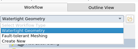
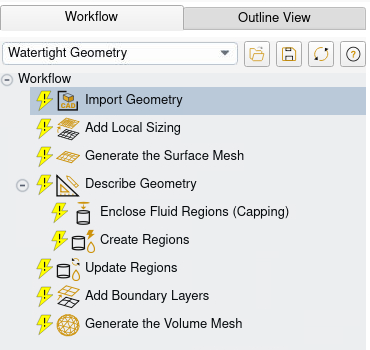
Each task is designated with an icon indicating its state (for example, as complete, incomplete, etc. All tasks are initially incomplete and you proceed through the workflow completing all tasks. Additional tasks are also available for the workflow.

2. Import the CAD geometry (manifold.pmdb)

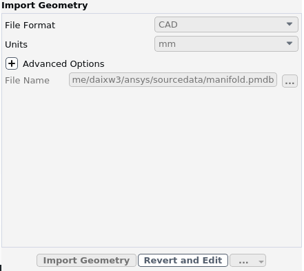
a. Select the Import Geometry task.

b. For File Format, keep the default setting of CAD.

c. For Units, keep the default setting as mm.

d. For File Name, enter the path and file name for the CAD geometry that you want to import (manifold.pmdb).

Note:

The workflow only supports *.scdoc (SpaceClaim),Workbench (.agdb), and the intermediary *.pmdb file formats.

The presentation version is based on *.pmdb files

e. Select Import Geometry.

This will update the task, display the geometry in the graphics window, and allow you to proceed onto the next task in the workflow.

Note:

Alternatively, you can use the ... button next to File Name to locate the CAD geometry file, after which, the Import Geometry task automatically updates, displaying the geometry in the graphics window, and the workflow automatically progresses to the next task.

Throughout the workflow, you are able to return to a task and change its settings using either the Edit button, or the Revert and Edit button.

3. Add local sizing

a. In the Add Local Sizing task, you are prompted as to whether or not you would like to add local sizing controls to the faceted geometry.

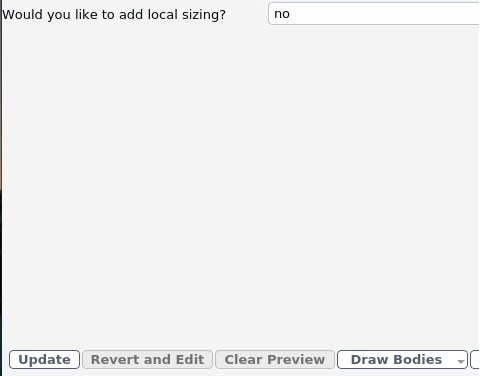
b. For the purposes of this tutorial, you can keep the default setting of no.

c. Click Update to complete this task and proceed to the next task in the workflow.

4. Generate the surface mesh

a. In the Generate the Surface Mesh task, you can set various properties of the surface mesh for the faceted geometry.

b. For the purposes of this tutorial, you can keep the default settings.

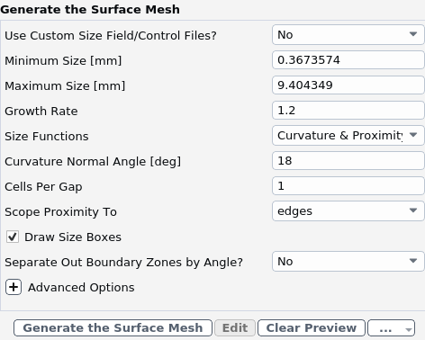
Note:

The red boxes displayed on the geometry in the graphics window are a graphical representation of size settings. These boxes change size as the values change, and they can be hidden by using the Clear Preview button.

c. Click Generate the Surface Mesh to complete this task and proceed to the next task in the workflow.

5. Describe the geometry

When you select the Describe Geometry task, you are prompted with questions relating to the nature of the imported geometry.

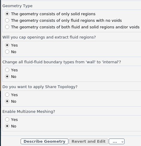
a. Since a fluid region is extracted from the solid model and capping surfaces are added, the default settings are appropriate.

b. Click Describe Geometry to complete this task and proceed to the next task in the workflow.

6. Cover any openings in your geometry

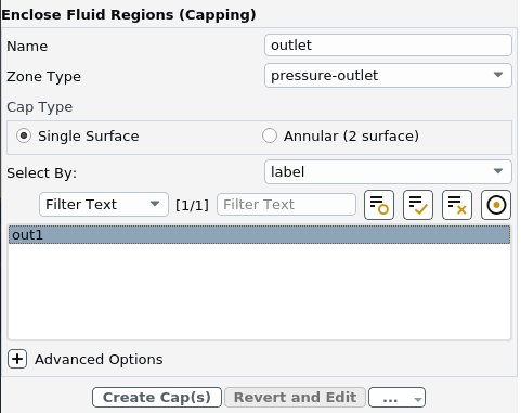
Select the Enclose Fluid Regions (Capping) task where you can cover or cap any openings in your geometry in order to later extract the enclosed fluid region.

a. Create a cap for the inlets.

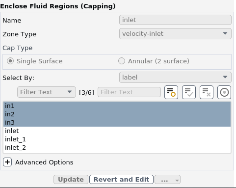
• In the Name field, assign a name for the capping surface (for example, inlet) to be assigned to all of the manifold's inlets.

• For the Zone Type, keep the default setting of velocity-inlet.

• For the Select By field, keep the default setting of label.

• In the list of labels, select in1, in2, and in3 for the openings that you want to cover.

  For occasions when the list of items is long, you can use the Filter Text option and use an expression such as in* to show only items starting with "in". Alternatively, you can use the Use Wildcard option to list and pres-select matching items. See Filtering Lists and Using Wildcards for more information.
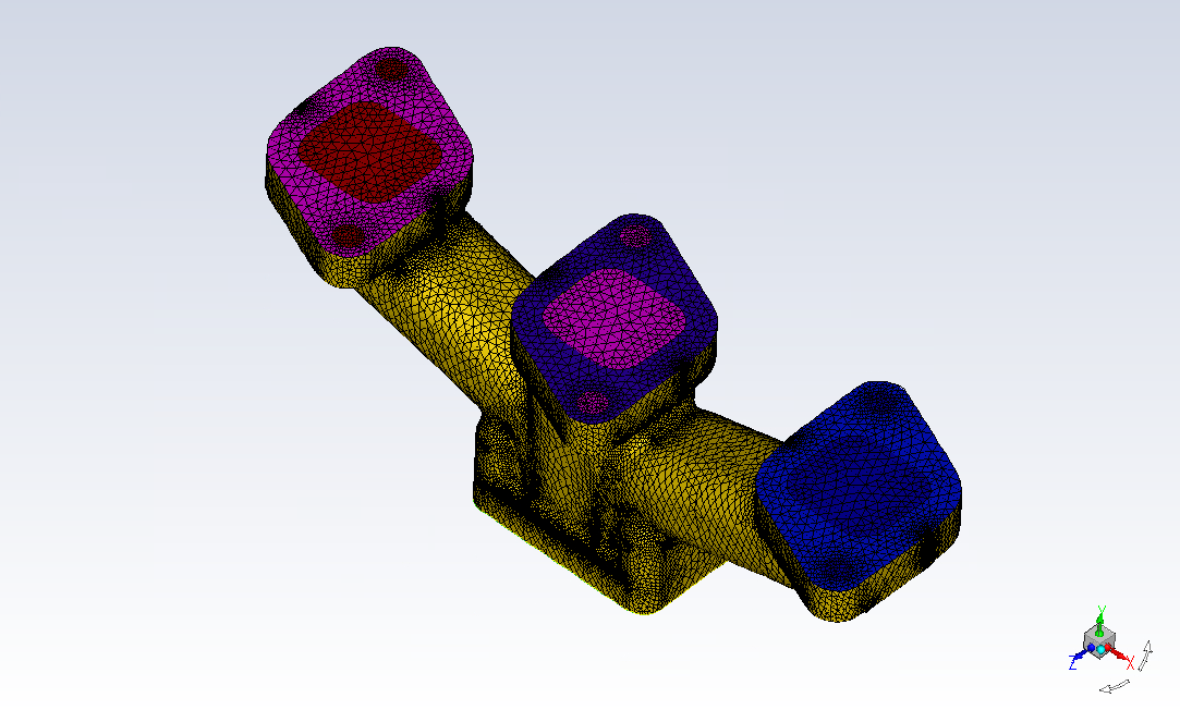
  The graphics window indicates the selected items.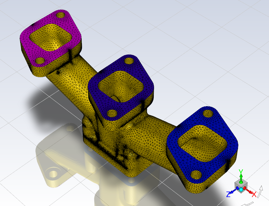
  

  

• Click Create Cap(s) to complete this task and proceed to the next task in the workflow.

b. Create a cap for the outlet.

• In the Name field, assign a name for the capping surface (for example, outlet) to be assigned to the manifold's outlet. For the Zone Type, change the setting to pressure-outlet.
• For the Select By field, keep the default setting of label.
• In the list of labels, select out1 for the outlet that you want to cover.
• Click Create Cap(s) to complete this task.

Now, all of the openings in the geometry are covered.

7. Create the fluid region

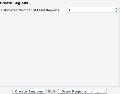
a. Select the Create Regions task, where you can determine the number of fluid regions that need to be extracted. Ansys Fluent attempts to determine the number of fluid regions to extract automatically.

b. For the Estimated Number of Fluid Regions, keep the default selection of 1.

c. Click Create Regions.

8. Update your regions

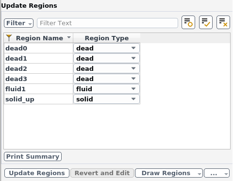
a. Select the Update Regions task, where you can review the names and types of the various regions that have been generated from your imported geometry, and change them as needed.

b. Keep the default settings, and click Update Regions.

xxxxxxxxxx
Aside from fluid regions and solid regions, you can also have voids within your geometry that are designated as dead regions. As you can see, there are four dead regions that correspond to the four bolt holes near the outlet, a solid region and a fluid region. Once the regions have been updated, the fluid region is displayed by default in the graphics window. You can use the Draw Regions button to display other options, such as drawing just the solid region, just the dead regions, or all regions.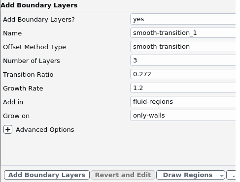

9. Add boundary layers

a. Select the Add Boundary Layers task, where you can set properties of the boundary layer mesh.

b. Keep the default settings, and click Add Boundary Layers.

10. Generate the volume mesh

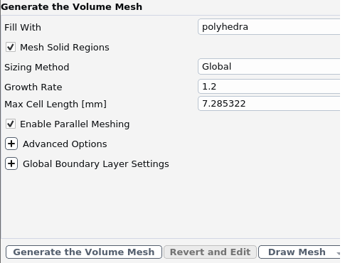
a. Select the Generate the Volume Mesh task, where you can set properties of the volume mesh.

b. Keep the default settings, and click Generate the Volume Mesh.

xxxxxxxxxx
Ansys Fluent will apply your settings and proceed to generate a volume mesh for the manifold geometry. Once complete, the mesh is displayed in the graphics window and a clipping plane is automatically inserted with a layer of cells drawn so that you can quickly see the details of the volume mesh.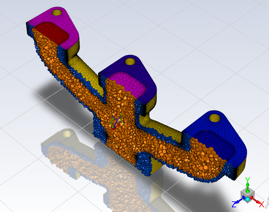

11. Save the mesh file

Mesh→ Check ，check the file.

File → Write → Mesh，save the mesh file

Setting the solution parameters

Now that a high-quality mesh has been generated using Ansys Fluent in meshing mode, you can now switch to solver mode to complete the set up of the simulation.

Switch to Solution mode.

We have just checked the mesh, so select Yes when prompted to switch to solution mode.

1. General Settings

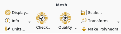
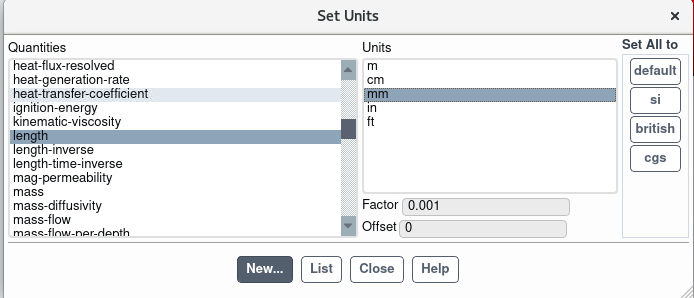
In the Mesh group box of the Domain ribbon tab, set the units for length..

Domain → Mesh → Units...

This opens the Set Units dialog box.

1. Select length under Quantities.
2. Select mm under Units.
3. Close the Set Units dialog box.

2. Solver Settings

In the Solver group box of the Physics ribbon tab, retain the default selection of the steady pressurebased solver.

Physics → Solver

3. Models

1. Set up your models for the CFD simulation using the Models group box of the Physics ribbon tab.

Note:

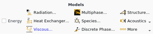
You can also use the Models task page, which can be accessed from the tree by expanding Setup and double-clicking the Models tree item.

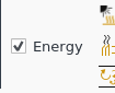
2. Enable heat transfer by activating the energy equation.

   Setup → Models → Energy On

3. Retain the default k-ω SST turbulence model.

   xxxxxxxxxx
   You will use the default settings for the k-ω SST turbulence model, so you can enable it directly from the tree by right-clicking the Viscous node and choosing SST k-omega from the context menu.
   

Setup → Models → Viscous(Right mouse click) → Model → SST k-omega

4. Materials

Change the default material of Aluminum to cast iron.

1. Create solid material properties for Cast Iron.

   Setup → Materials → Solid → Aluminum(Right mouse click) → Edit...

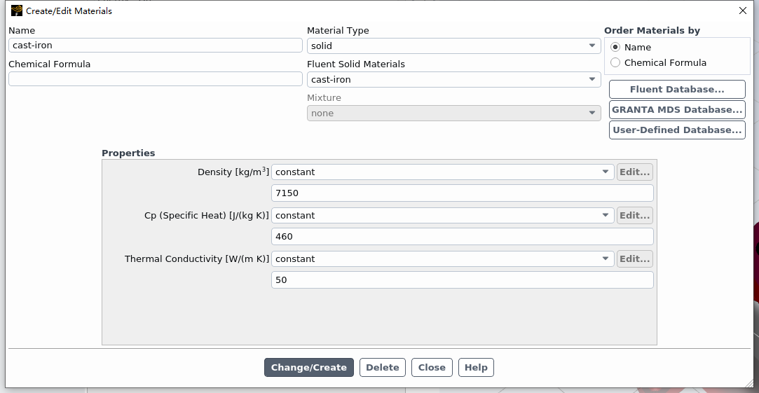
a. Change the name of the material to be cast-iron.

b. Clear the Chemical Formula field.

c. Change the Density to 7150 kg/m3.

d. Change the Cp to 460 j/kg-k.

e. Change the Thermal Conductivity to 50 w/m-k.

f. Click Change/Create and overwrite the Aluminum material.

g. Click Yes to replace the Aluminum material.

h. Close the Create/Edit Materials dialog box.

5. Cell Zone Conditions

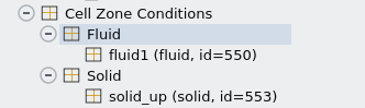
Ordinarily, you would set up the cell zone conditions for the CFD simulation using the Zones group box of the Physics ribbon tab. The properties of air for the fluid zone and cast-iron for the solid zone will be used.

6. Boundary Conditions

1.Set the velocity, turbulence, and thermal boundary conditions for the first inlet (inlet).

Setup → Boundary Conditions → Inlet → inlet(Right mouse click) → Edit...

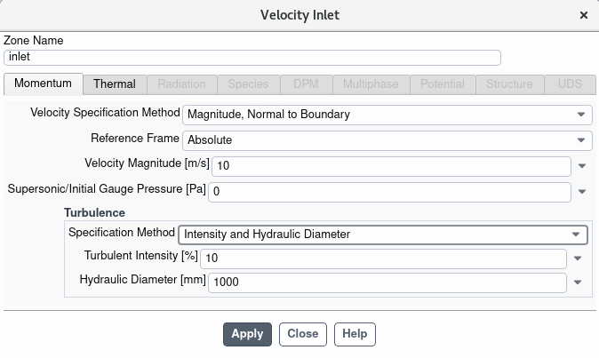
a. Enter 10 m/s for Velocity Magnitude.

b. In the Turbulence group box, select Intensity and Hydraulic Diameter from the Specification Method drop-down list.

c. Enter 10 % for the Turbulent Intensity.

d. Enter 40 mm for the Hydraulic Diameter.

e. Click the Thermal tab

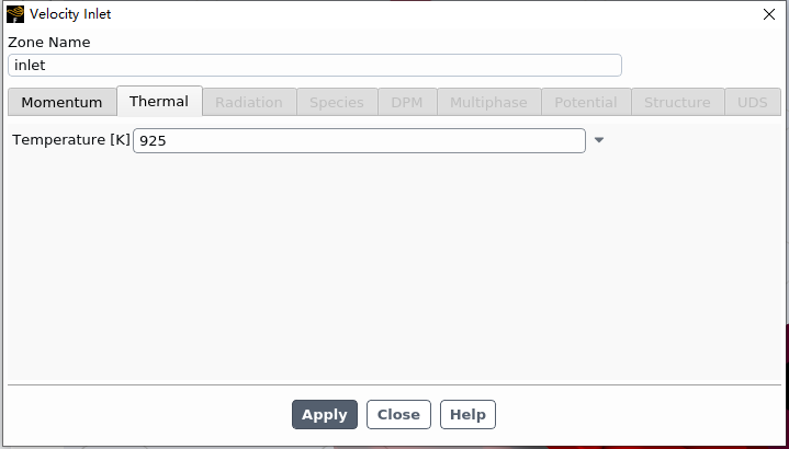
f. Enter 925 [K]

g. Click Apply and close the Velocity Inlet dialog box.

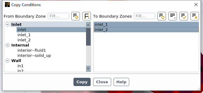
2.Apply the same conditions to the other inlets (inlet1, and inlet2).

a. Select inlet from the Boundary Conditions node of the Outline View, right-click and select Copy from the context menu.

This opens the Copy Conditions dialog box.

b. Select inlet _1 and inlet_2 from the To Boundary Zones list. c. Click Copy, click OK in the confirmation prompt, and close the Copy Conditions dialog box.

3.Set the boundary conditions at the outlet (outlet).

Setup → Boundary Conditions → Outlet → outlet(Right mouse click) → Edit...

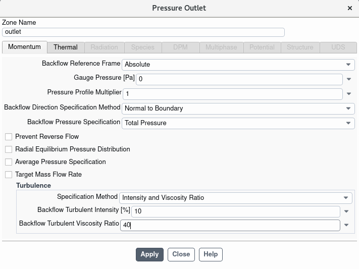
a. Retain the default setting of 0 for Gauge Pressure.

b. In the Turbulence group box, select Intensity and Hydraulic Diameter from the Specification Method drop-down list.

c. Retain the default value of 10% for the Backflow Turbulent Intensity.

d. Enter 40 mm for the Backflow Hydraulic Diameter.

e. Click Apply and close the Pressure Outlet dialog box.

4.Set the wall heat transfer boundary conditions. Setup → Boundary Conditions → Wall → solid_up:1(Right mouse click) → Edit...

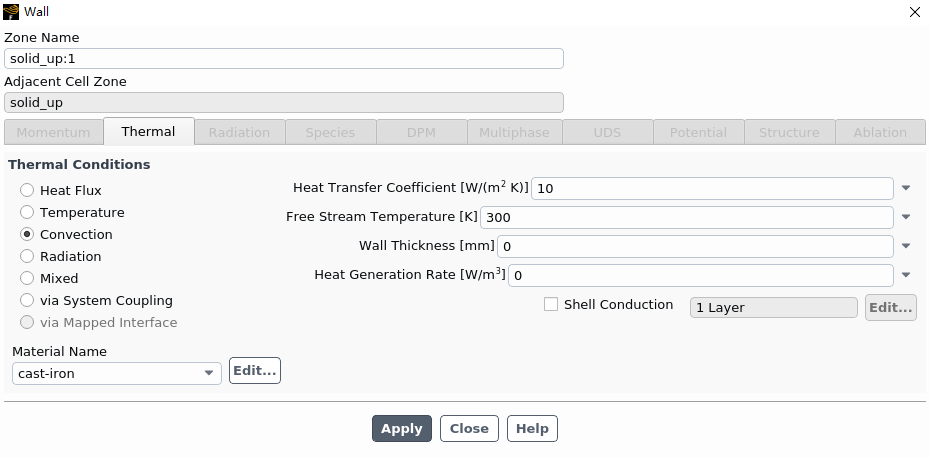
a. Select Convection under Thermal Conditions.

b. Enter 10 for the Heat Transfer Coefficient.

c. Enter 300 for the Free Stream Temperature.

d. Click Apply and close the Wall dialog box.

5.Apply the same conditions to the other walls (in1, in2, in3, and out1).

a. Select solid_up:1 from the Boundary Conditions node of the Outline View, right-click and select Copy from the context menu.

This opens the Copy Conditions dialog box.

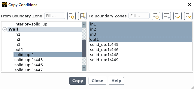
b. Select in1, in2, in3, and out1 from the To Boundary Zones list.

c. Click Copy, click OK in the confirmation prompt, and close the Copy Conditions dialog box.

6.Retain the remaining default (wall and interior) boundary conditions.

7. Solution

1.Specify the discretization schemes. In the Solution ribbon tab, click Methods... (Solution group box).

Solution → Solution → Methods...

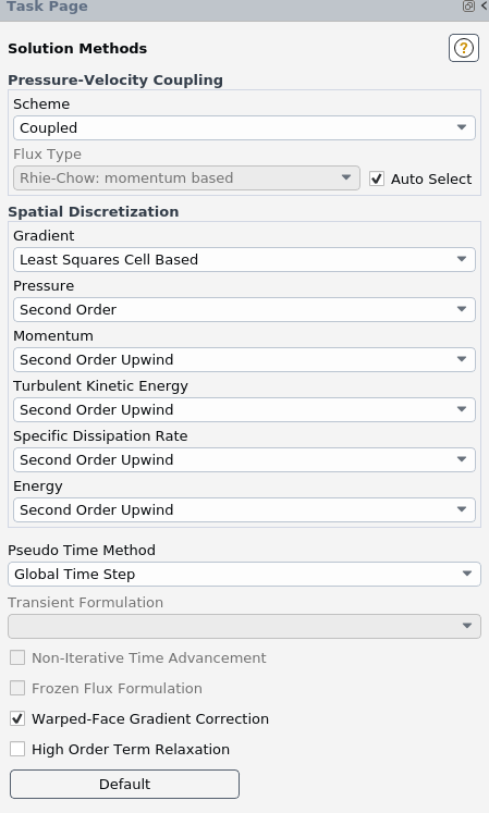
Retain the default settings.

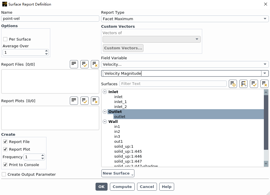
2.Create a surface report definition of the velocity at the outlet (outlet).

Solution → Reports Definitions → New → Surface Report → Facet Maximum...

Note: You can also access the Surface Report Definition dialog box by right-clicking Report Definitions in the tree (under Solution) and selecting New/Surface Report/Facet Maximum... from the menu that opens.

a. Enter point-vel for the Name of the report definition.

b. Enable Report File, Report Plot, and Print to Console in the Create group box.

xxxxxxxxxx
During a solution run, Ansys Fluent will write solution convergence data in a report file, plot the solution convergence history in a graphics window, and print the value of the report definition to the console.

c. Select Velocity... and Velocity Magnitude from the Field Variable drop-down lists.

d. Select outlet from the Surfaces selection list.

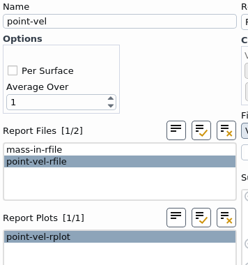
e. Click OK to save the surface report definition and close the Surface Report Definition dialog box.

The new surface report definition point-vel will appear under the Solution/Report Definitions tree item. Ansys Fluent also automatically creates the following items: • point-vel-rfile (under the Solution/Monitors/Report Files tree branch) • point-vel-rplot (under the Solution/Monitors/Report Plots tree branch)

3.Monitor the mass flow rate at the inlets.

Solution → Reports Definitions → New → Flux Report → Mass Flow Rate...

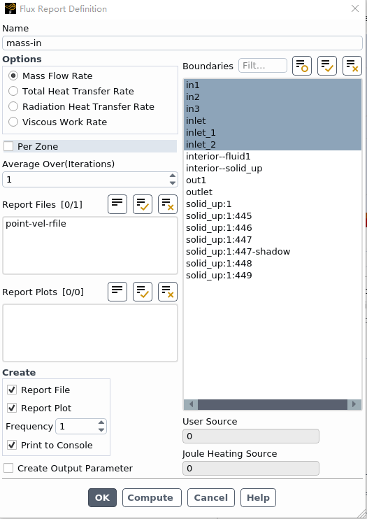
a. Enter mass-in for the Name of the report definition.

b. Select Mass Flow Rate under Options.

c. Select in1, in2, in3, as well as inlet, inlet_1, inlet_2 from the Boundaries selection list.

d. Enable Report File, Report Plot, and Print to Console in the Create group box.

e. Click OK to save the surface report definition and close the Flux Report Definition dialog box.

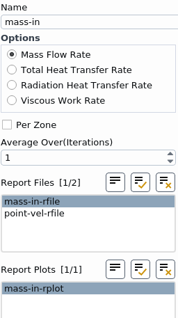
The new surface report definition mass-in will appear under the Solution/Report Definitions tree item. Ansys Fluent also automatically creates the following items: • mass-in-rfile (under the Solution/Monitors/Report Files tree branch) • mass-in-rplot (under the Solution/Monitors/Report Plots tree branch)

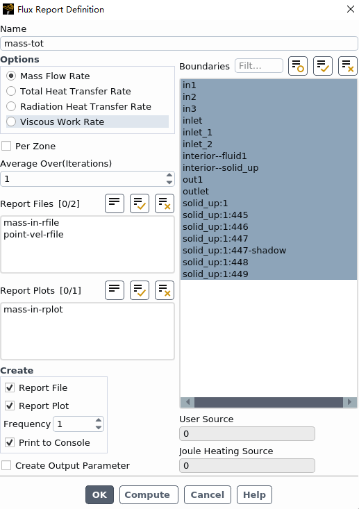
4.Monitor the total mass flow rate through the entire domain.

Perform the same procedure as described above, naming the report mass-tot, and selecting all boundaries.

5.Monitor the mass balance.

Use expressions to create a report definition for the mass balance using existing report definitions.

Solution → Reports → Definitions → New → Expression...

This opens the Expression Report Definition dialog box.

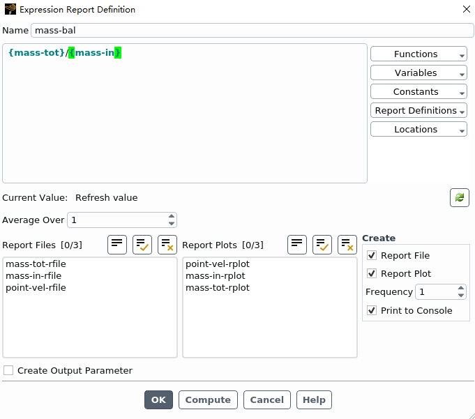
a. Enter mass-bal for the Name of the expression.

b. Select mass-tot from the Report Definitions drop-down list on the right.

c. Type the / operand.

d. Select mass-in from the Report Definitions drop-down list on the right.

e. Enable Report File, Report Plot, and Print to Console in the Create group box.

f. Click OK to save the expression definition.

6.Initialize the flow field using the Initialization group box of the Solution ribbon tab.

Solution → Initialization

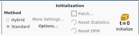
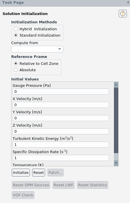
a. Select Standard from the Method list.

b. Click Initialize.

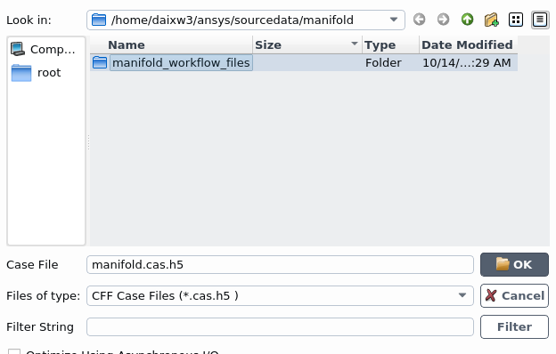
7.Save the case file (manifold_solution.cas.h5).

File → Write → Case...

Preprocessing completed

ANSYS Fluent Postprocessing Example

1.Display path lines highlighting the flow field.

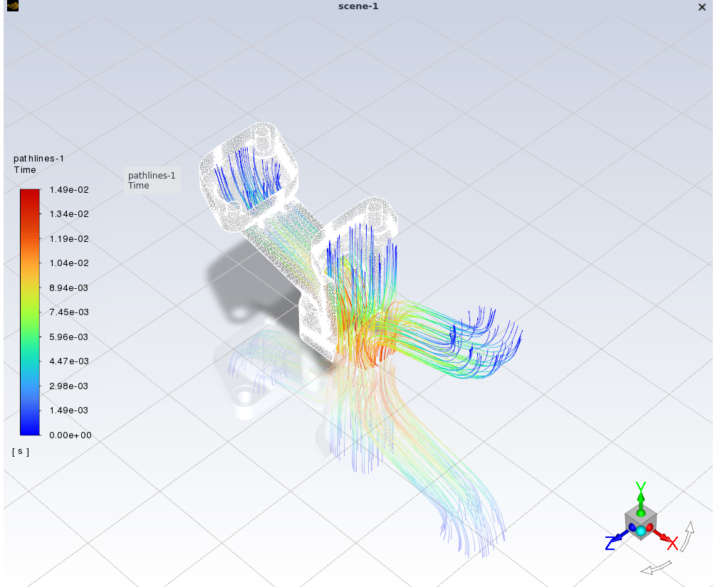
Results → Graphics → Pathlines → New...

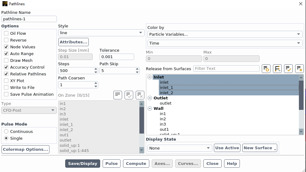
a. Keep the default of pathlines-1 for the Name.

b. Select Particle Variables... and Time from the Color by drop-down lists.

c. Set the Path Skip value to 5.

d. Select Accuracy Control from the Options list.

e. Select inlet, inlet_1, and inlet_2 from the Release from Surfaces list.

f. Click Save/Display and close the Pathlines dialog box.

xxxxxxxxxx
The new pathlines-1 definition appears under the Results/Graphics/Pathlines tree branch. To edit your surface definition, right-click it and select Edit... from the menu that opens.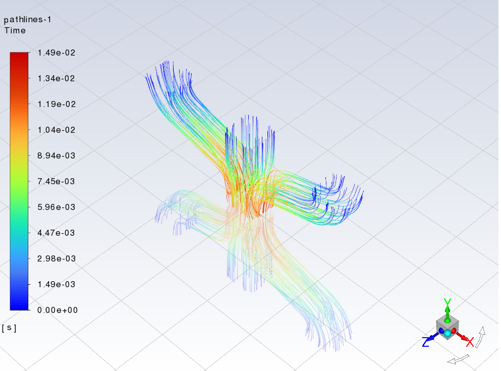

2.Create two clipped surfaces through the manifold geometry.

Results → Surface → Create → Iso-Clip...

a. Create Surface 1

• Enter clip-x-coordinate for Name.
• Select Mesh... and X-Coordinate from the Clip to Values of drop-down lists.
• Select solid_up:1 from the Clip Surface list.
• Click Compute.
• Keep the Min value at its minimum setting, and adjust the Max value to be at its halfway point.
• Click Create.

xxxxxxxxxx
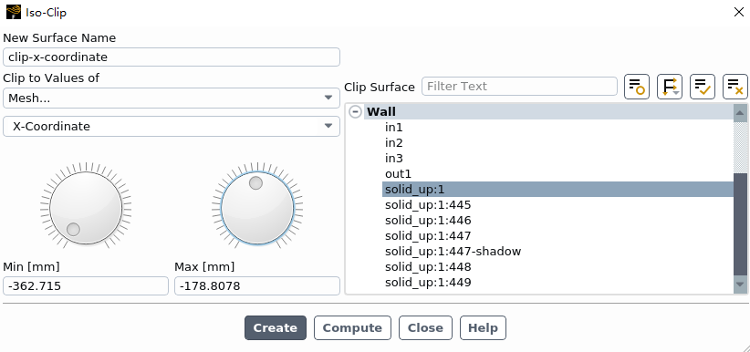
The new clip-x-coordinate definition appears under the Results/Surfaces tree branch. To edit your surface definition, right-click it and select Edit... from the menu that opens.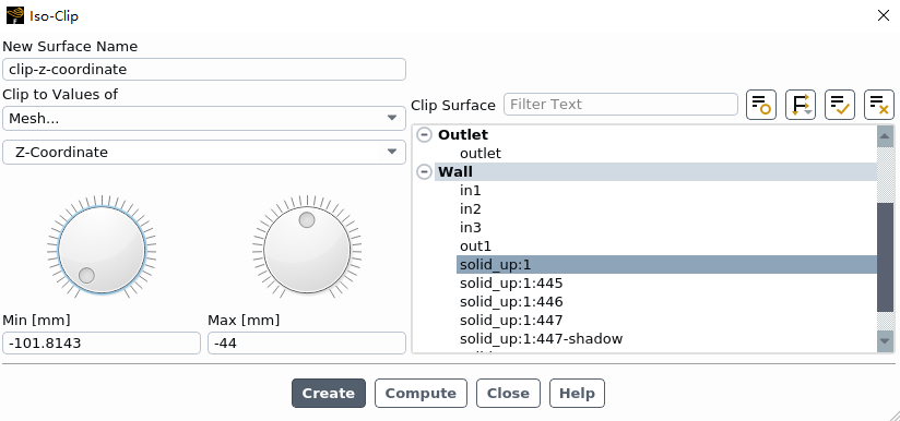

b. Create Surface 2

• Enter clip-z-coordinate for Name.
• Select Mesh... and Z-Coordinate from the Clip to Values of drop-down lists.
• Select solid_up:1 from the Clip Surface list.
• Click Compute.
• Keep the Min value at its minimum setting, and adjust the Max value to be at -44.0 .
• Click Create and close the Iso-Clip dialog box.

xxxxxxxxxx
The new clip-z-coordinate definition appears under the Results/Surfaces tree branch. To edit your surface definition, right-click it and select Edit... from the menu that opens.

3.Create a scene containing the mesh and the path lines.

Results → Scene(Right mouse click) → New...

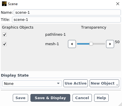
a. Keep the default scene-1 for the Name.

b. Enable the pathlines-1 graphics object.

c. Create a new mesh object to add to the scene.

• Click New Object and select Mesh to open the Mesh Display dialog box.

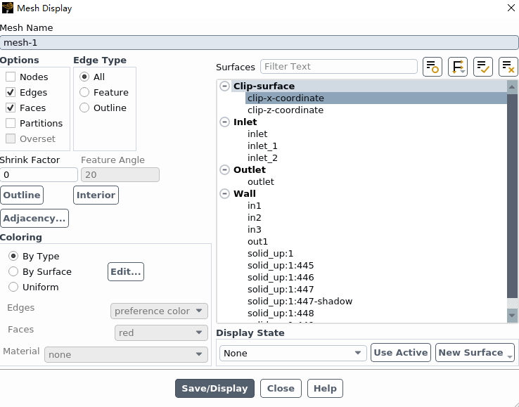
• Ensure that Edges is selected under the Options list.
• Select clip-x-coordinate under the Surfaces list.
• Click Save/Display and close the Mesh Display dialog box.

xxxxxxxxxx
The new mesh-1 definition appears under the Results/Graphics/Mesh tree branch. The new object also appears in the Scene dialog box.

d. In the Scene dialog box, set the Transparency of mesh-1 to 50.

e. Click Save & Display and close the Scene dialog box.

4.Create and define contours of velocity magnitude at the outlet along with the mesh.

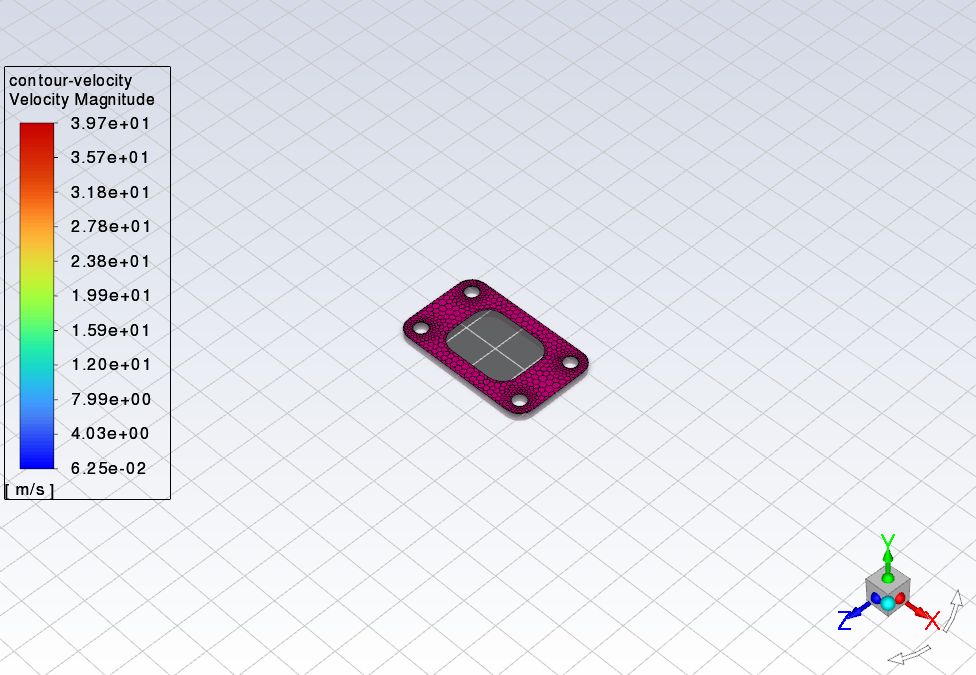
Results → Graphics → Contours → New...

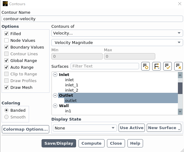
a. Enter contour-velocity for the Name.

b. Select Velocity... and Velocity Magnitude from the Contours of drop-down lists.

c. Select outlet from the Surfaces list.

d. Disable Node Values under Options.

e. Enable Draw Mesh under Options.

This displays the Mesh Display dialog box.

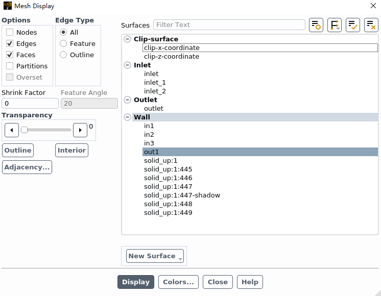
In the Mesh Display dialog box, deselect all surfaces, select the out1 surface, click Display and close the dialog.

f. Click Save/Display and close the Contours dialog box.

5.Create an iso-surface through the manifold geometry.

Results → Surface → Create → Iso-Surface...

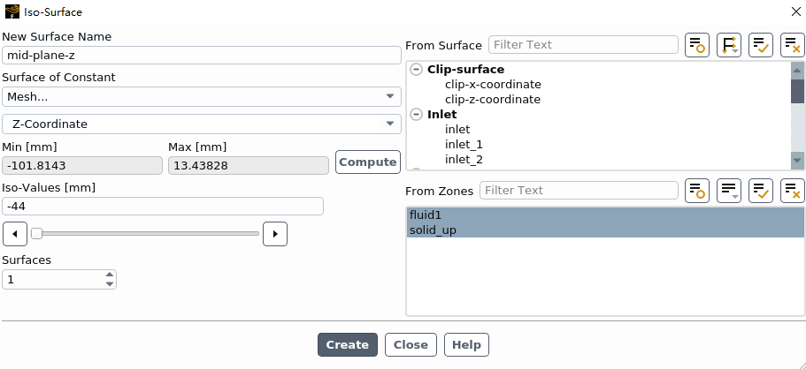
a. Enter mid-plane-z for Name.

b. Select Mesh... and Z-Coordinate from the Surface of Constant drop-down lists.

c. Select fluid1 and solid_up from the From Zones... list.

d. Click Compute.

The Min and Max fields display the Z extents of the domain.

e. Enter 44 for the Iso-Values.

f. Click Create and close the Iso-Surface dialog box.

6.Create and define a contour of temperature along the mid-plane.

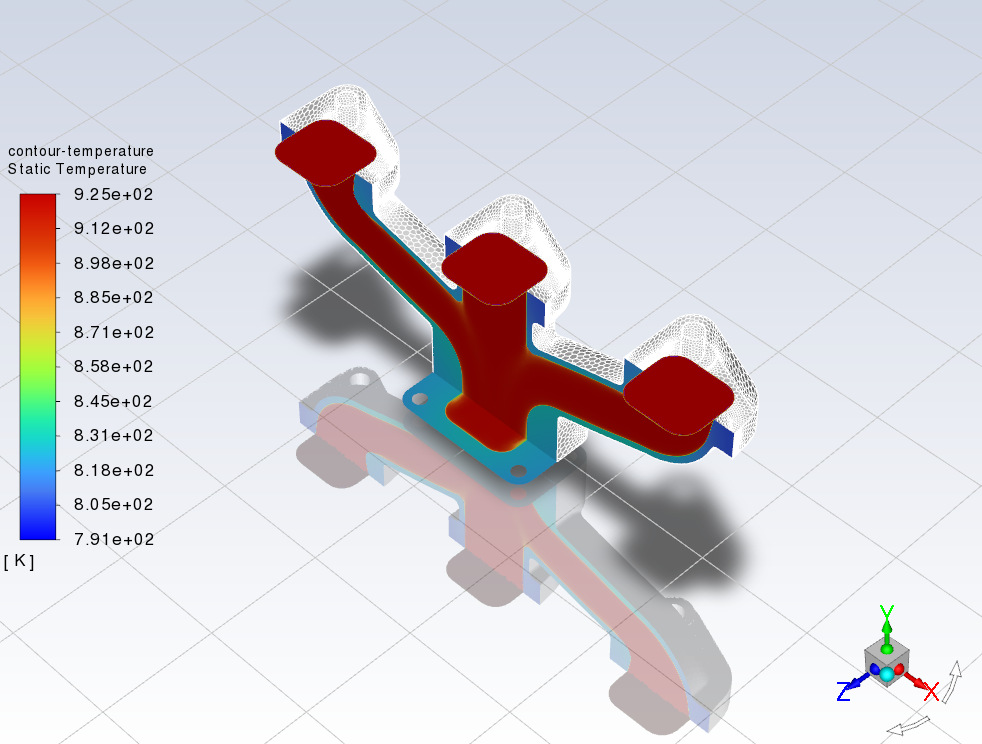
Results → Graphics → Contours → New...

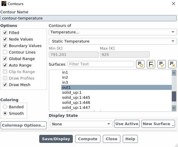
a. Enter contour-temperature for the Name.

b. Select Temperature... and Static Temperature from the Contours of drop-down lists.

c. Select inlet, inlet_1, inlet_2, mid-plane-z, outlet, and out1 from the Surfaces list.

d. Enable Draw Mesh under Options.

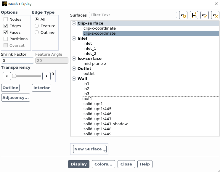
In the Mesh Display dialog box, deselect all surfaces, select the clip-z-coordinate surface, click Display and close the dialog.

e. Click Save/Display and close the Contours dialog box.

7.Create and define a contour of temperature for the manifold geometry.

Results → Graphics → Contours → New...

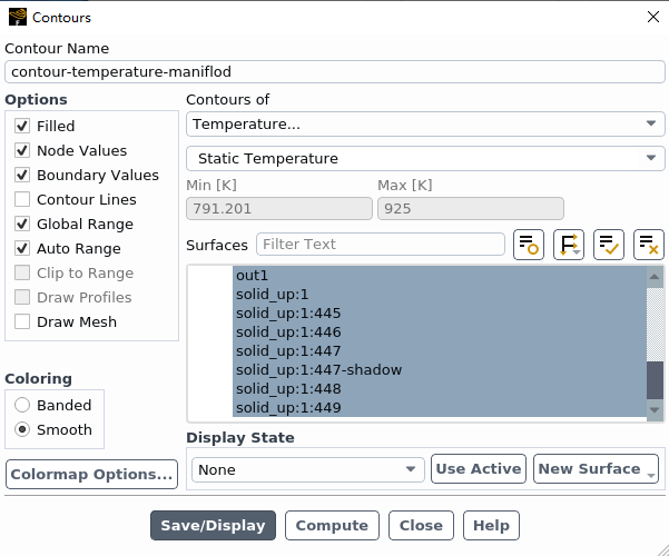
a. Enter contour-temperature-manifold for the Name.

b. Select Temperature... and Static Temperature from the Contours of drop-down lists.

c. Select the Wall group from the Surfaces list.

d. Click Save/Display and close the Contours dialog box.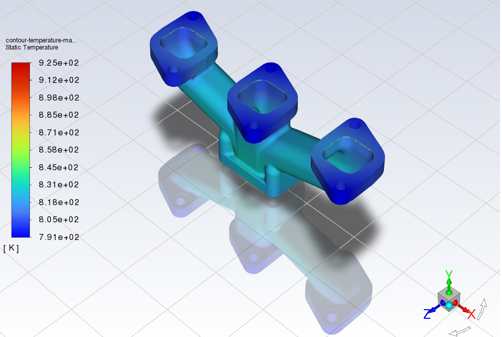

8.Save the case and data files (manifold_solution.cas.h5 and manifold_solution.dat.h5).

File → Write → Case & Data...

Save the files for post-processing

Post-processing completed